Data Frofilling Report
24 Oct 2019
Overview
The notebook aims to:
- Import data and load libraries
- Generate a prescriptive EDA repot
Load libraries
library(skimr)          # summary stats
library(DataExplorer)   # variable profiling, EDA
library(tidyverse)      # data manipulation
library(tidymodels)     # modelling
library(highcharter)    # interactive visualization
library(janitor)        # clean column names, convert to snake case
Import data
dat <- read_csv(params$dpath) %>%
  rename(target = params$target_name) %>%
  clean_names()
dim(dat)
## [1] 506 14Summary statistics
dat %>% skim_to_wide() %>% kable()| type | variable | missing | complete | n | mean | sd | p0 | p25 | p50 | p75 | p100 | hist |
|---|---|---|---|---|---|---|---|---|---|---|---|---|
| numeric | age | 0 | 506 | 506 | 68.57 | 28.15 | 2.9 | 45.02 | 77.5 | 94.07 | 100 | ▁▂▂▂▂▂▃▇ |
| numeric | b | 0 | 506 | 506 | 356.67 | 91.29 | 0.32 | 375.38 | 391.44 | 396.23 | 396.9 | ▁▁▁▁▁▁▁▇ |
| numeric | chas | 0 | 506 | 506 | 0.069 | 0.25 | 0 | 0 | 0 | 0 | 1 | ▇▁▁▁▁▁▁▁ |
| numeric | crim | 0 | 506 | 506 | 3.61 | 8.6 | 0.0063 | 0.082 | 0.26 | 3.68 | 88.98 | ▇▁▁▁▁▁▁▁ |
| numeric | dis | 0 | 506 | 506 | 3.8 | 2.11 | 1.13 | 2.1 | 3.21 | 5.19 | 12.13 | ▇▅▃▃▂▁▁▁ |
| numeric | indus | 0 | 506 | 506 | 11.14 | 6.86 | 0.46 | 5.19 | 9.69 | 18.1 | 27.74 | ▃▆▅▁▁▇▁▁ |
| numeric | lstat | 0 | 506 | 506 | 12.65 | 7.14 | 1.73 | 6.95 | 11.36 | 16.96 | 37.97 | ▆▇▆▅▂▁▁▁ |
| numeric | nox | 0 | 506 | 506 | 0.55 | 0.12 | 0.38 | 0.45 | 0.54 | 0.62 | 0.87 | ▇▆▇▆▃▅▁▁ |
| numeric | ptratio | 0 | 506 | 506 | 18.46 | 2.16 | 12.6 | 17.4 | 19.05 | 20.2 | 22 | ▁▂▂▂▅▅▇▃ |
| numeric | rad | 0 | 506 | 506 | 9.55 | 8.71 | 1 | 4 | 5 | 24 | 24 | ▂▇▁▁▁▁▁▅ |
| numeric | rm | 0 | 506 | 506 | 6.28 | 0.7 | 3.56 | 5.89 | 6.21 | 6.62 | 8.78 | ▁▁▂▇▇▂▁▁ |
| numeric | target | 0 | 506 | 506 | 22.53 | 9.2 | 5 | 17.02 | 21.2 | 25 | 50 | ▂▅▇▆▂▂▁▁ |
| numeric | tax | 0 | 506 | 506 | 408.24 | 168.54 | 187 | 279 | 330 | 666 | 711 | ▃▇▂▅▁▁▁▆ |
| numeric | zn | 0 | 506 | 506 | 11.36 | 23.32 | 0 | 0 | 0 | 12.5 | 100 | ▇▁▁▁▁▁▁▁ |
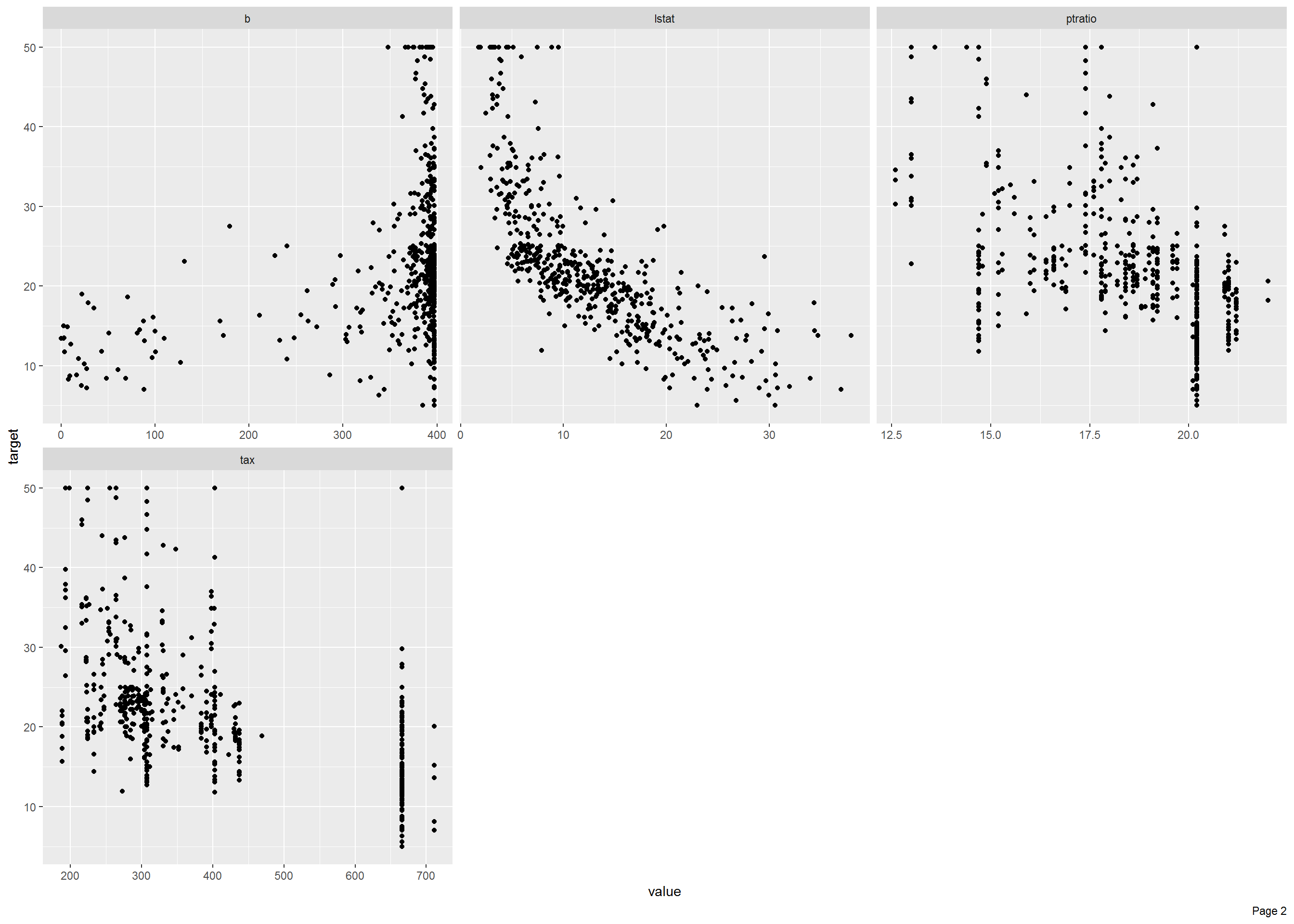
Univariate Plots
plot_boxplot(dat, by = "target")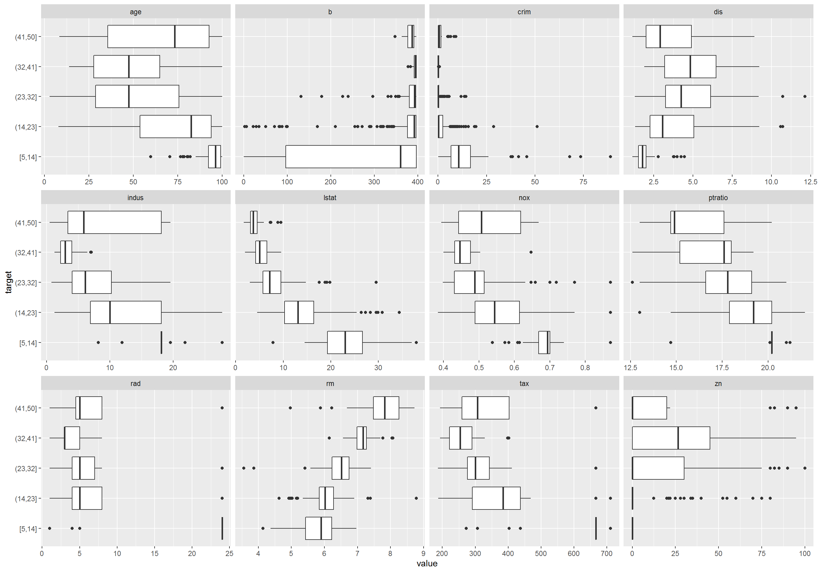
plot_scatterplot(dat, by = "target")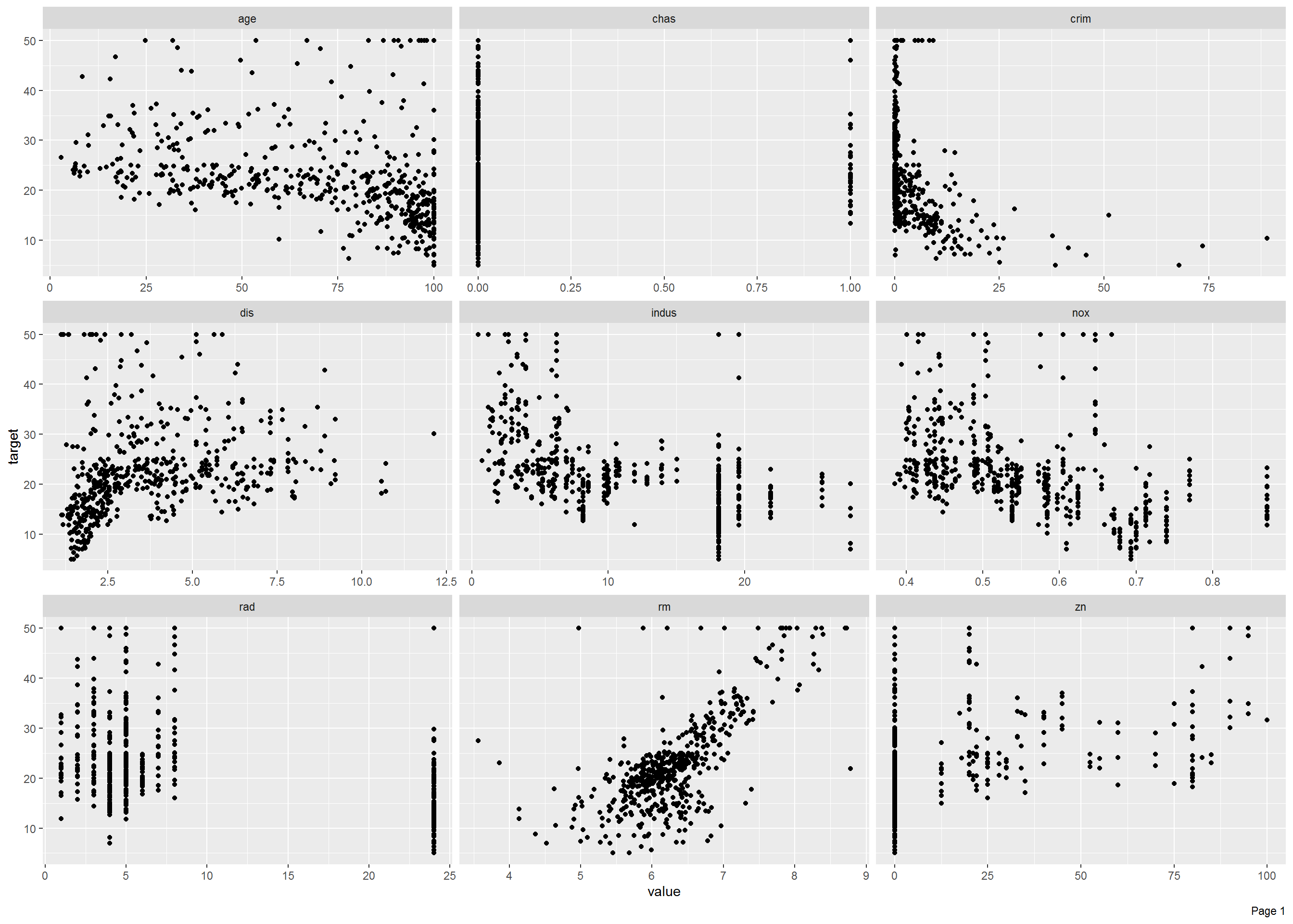
Correlation Heatmap
dat %>%
  select_if(rlang::is_bare_numeric) %>%
  cor() %>%
  GnT::hchart_cor()